Quantum Chemistry Part 2

Introduction
Chemistry
Author

NicDeclic

Published

October 14, 2026

“Your only adversary is the mirror that refuses to reflect all your colors.”
— Professor Alvin


Click to see library imports
import sys
if 'google.colab' in sys.modules:
    # 1. Download qmc.py from GitHub
    !wget -q https://raw.githubusercontent.com/nicdeclic/quantum-molecular-computing/main/qmc.py
    
    # 2. Download requirements.txt from GitHub
    !wget -q https://raw.githubusercontent.com/nicdeclic/quantum-molecular-computing/main/requirements.txt

    # 3. Install dependencies
    !pip install -q -r requirements.txt

sys.path.insert(0, "../../src") # Select root directory
from qmc import * # QMC library

%reload_ext autoreload
%autoreload 2

Closed Form Molecules

Code
# Create a conjugated carbon molecule
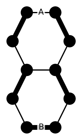
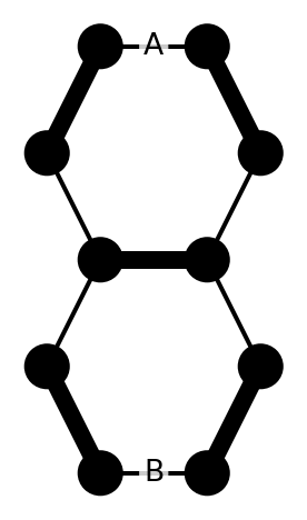
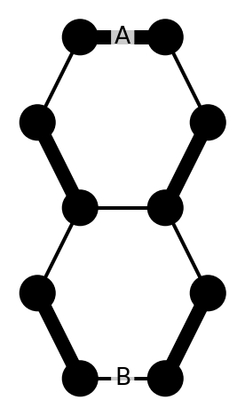
mol1 = CarbonMolecule("Double Honeycomb")

# Add atoms
c1_1 = mol1.add_atom(x=-0.25, y=1)
c1_2 = mol1.add_atom(x=0.25, y=1)
c1_3 = mol1.add_atom(x=-0.5, y=0.5)
c1_4 = mol1.add_atom(x=0.5, y=0.5)
c1_5 = mol1.add_atom(x=-0.25, y=0)
c1_6 = mol1.add_atom(x=0.25, y=0)
c1_7 = mol1.add_atom(x=-0.5, y=-0.5)
c1_8 = mol1.add_atom(x=0.5, y=-0.5)
c1_9 = mol1.add_atom(x=-0.25, y=-1)
c1_10 = mol1.add_atom(x=0.25, y=-1)

# Add bonds
b1_1 = mol1.add_bond(c1_1, c1_2, order="single", label="A", role="input")
b1_2 = mol1.add_bond(c1_2, c1_4, order="single")
b1_3 = mol1.add_bond(c1_1, c1_3, order="single")
b1_4 = mol1.add_bond(c1_3, c1_5, order="single")
b1_5 = mol1.add_bond(c1_4, c1_6, order="single")
b1_6 = mol1.add_bond(c1_5, c1_6, order="single")
b1_7 = mol1.add_bond(c1_5, c1_7, order="single")
b1_8 = mol1.add_bond(c1_6, c1_8, order="single")
b1_9 = mol1.add_bond(c1_7, c1_9, order="single")
b1_10 = mol1.add_bond(c1_8, c1_10, order="single")
b1_11 = mol1.add_bond(c1_9, c1_10, order="single", label="B", role="output")

# Draw with Schemdraw
# mol1.draw()

all_resonances = mol1.resonance()

for i, res_mol in enumerate(all_resonances):
    res_mol.draw() 

Code
CarbonMolecule.resonance_table(all_resonances)

\[\begin{array}{|c|c|} \hline \mathbf{A} & \mathbf{B} \\ \hline 0 & 1 \\ 0 & 0 \\ 1 & 0 \\ \hline \end{array}\]

Classical boolean logic provides no native vocabulary to express such non-uniform states.

Deterministic certainty dissolves here. We are forced to broaden our theoretical horizons into statistics.


Probabilistic Bits (p-bits)

Probabilistic bits provide a robust mathematical framework for encoding and processing information. By applying this formalism to carbon-carbon bonds, we can natively capture the stochastic nature of chemical systems and open up new frontiers in molecular computing.

Think of a coin toss. Once flipped, the coin can land on tails (state “0”) or heads (state “1”).

With a fair coin, there is an equal probability—a 50% chance—of landing on state “0” and a 50% chance of landing on state “1”.

Mathematically, we formulate probabilistic bits using the same transition matrices introduced earlier. The only operational difference lies in the values of the matrix elements.

  • A fair coin: :
Code
display_inline("Fair", "=", random.to_katex(show_labels=True))

\[ Fair = \begin{array}{r|cc|} \text{} & \text{``0''} & \text{``1''} \\ \hline ~ & 0.5 & 0.5 \\ \hline \end{array} \]

The first element quantifies the probability of observing a “0”; the second element quantifies the probability of observing a “1”.

We could also bias the coin so that it carries a one-in-four chance (25%) of landing on “0”, and a three-in-four chance (75%) of landing on “1”.

  • A biased coin: :
Code
biased = TransitionMatrix([
    [0.25, 0.75]
])

display_inline("Biased", "=", biased.to_katex(show_labels=True))

\[ Biased = \begin{array}{r|cc|} \text{} & \text{``0''} & \text{``1''} \\ \hline ~ & 0.25 & 0.75 \\ \hline \end{array} \]

The limiting boundary case occurs when there is a 0% chance of being in one state and a 100% chance of being in the other. Under these conditions, deterministic certainty is recovered, and the probabilistic bit collapses back into a classical boolean bit.

Any continuous probability distribution is physically admissible, provided that two fundamental axioms are satisfied:
1. Every individual element must lie strictly within the closed interval \([0, 1]\).
2. The elements along each row must sum to exactly 1 (equivalent to 100%—the total probability space). Consequently, there is no probability leak into unmodeled states (for example, ruling out the pathological edge case where the coin lands balanced on its side).

And because of the missing row values we must add a third axiom:

  1. The elements along a row representing an invalid state must sum to exactly 0 (dead-end).

Code
doubleHoneycomb = TransitionMatrix.from_resonances(all_resonances)

display_inline("DoubleHoneycomb", "=", doubleHoneycomb.to_katex(show_labels=True))

\[ DoubleHoneycomb = \begin{array}{r|cc|} \text{} & \text{``0''} & \text{``1''} \\ \hline \text{``0''} & 0.5 & 0.5 \\ \text{``1''} & 1 & 0 \\ \hline \end{array} \]


The Breakthrough

  • NOR gate.

Double Connections


Cascading Parasitic Resonance (Molecular Epilepsy)

When a junction allows two unauthorized boundary states to infiltrate its truth table, these spurious modes do not remain localized. They infect adjacent nodes, triggering what we might call Cascading Parasitic Resonance — or, in more intuitive neuro-computational terms, a form of molecular epilepsy sweeping across the quantum network.


Couplers


Reverse Computing

  • Transpose operation.

  • The resonance states must be bijective.


Speculations & Wild Thoughts

  • If biological neural networks rely on aromatic π-electron resonance networks within synaptic receptors for ultrafast signaling, what happens when a molecular coupler suffers a geometric defect?
    Could an epileptic seizure be the macroscopic manifestation of a microscopic state - leakage cascade—where the breakdown of a single quantum molecular parity check forces millions of synapses into a runaway, hypersynchronous parasitic resonance?
👉 Next chapter :
“The Emergence of Protobits”