Gates like the Hadamard gate and the T gate, are fundamentally more complex. Geometrically, they rotate the state to points that lie between the vertices—on the faces or edges of the Bloch sphere. They cannot be implemented by a simple one-to-one permutation of discrete vertices.
The Pauli gates (\(X, Y, Z\)) and the phase gate (\(S\)) were straightforward because every vertex of our 8-state cube mapped cleanly and deterministically onto another single vertex.
Gates like the Hadamard gate (\(H\)) and the \(T\) gate (\(\pi/8\) rotation), however, are fundamentally more complex. Geometrically, they rotate the state to points that lie between the vertices—on the faces or edges of the Bloch sphere. They cannot be implemented by a simple one-to-one permutation of discrete vertices.
The Hadamard Gate
The Hadamard gate is the quintessential quantum superposition operator. In the standard Dirac computational basis, it maps basis states into equal linear combinations:
Notice a remarkable mathematical symmetry: the Hadamard matrix can be decomposed exactly as the normalized sum of the \(X\) and \(Z\) Pauli operators:
\[H = \frac{1}{\sqrt{2}} (X + Z)\]
This identity provides our architectural blueprint!
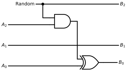
We can synthesize the Hadamard transformation by:
1. Routing our input protobit triplet \((A_2, A_1, A_0)\) into both the \(X\) circuit and the \(Z\) circuit in parallel.
2. Superposing the output channel selection using a fair-coin random source to balance the branches with equal probability weights.
By leveraging physical resonance and stochastic mixing, the discrete geometry of protobits natively recreates the continuous superposition of the Hadamard transform.
Don’t forget that the boolean logic gates depicted below operate as native quantum transition operators capable of manipulating coherent protobit states.
Additionally, the Random signal is entirely internal to the gate’s molecular framework—acting as a local stochastic fluctuation rather than an external control line—so there is no need to route it from outside the cell.
Code
# Initialize schematic drawing for the Hadamard circuitwith schemdraw.Drawing() as d: d.config(fontsize=12, unit=2.5)# Vertical coordinates for the rails y_rand =4.5 y_a2 =3.0 y_a1 =1.5 y_a0 =0.0 x_in =0.0# ==========================================# 1. Logic Gates Setup# ==========================================# AND gate: inputs from Random and A2 and_gate = d.add(logic.And().right().at((3.0, 3.25)))# XOR gate: inputs from AND output and A0 -> drives B0 xor_gate = d.add(logic.Xor().right().at((5.0, y_a0 +0.25)))# ==========================================# 2. Random Source Line -> Drives B2 and AND gate# ========================================== d.add( elm.Line() .right(6.0) .at((x_in +2, y_rand)) .label("Random", loc="left") .label("$B_2$", loc="right") )# Branch down to AND gate input 1 d.add(elm.Dot().at((2.5, y_rand))) d.add(elm.Wire("|-").at((2.5, y_rand)).to(and_gate.in1))# ==========================================# 3. Input A2 Line -> Drives AND gate input 2# ========================================== d.add( elm.Line() .at((x_in, y_a2)) .to(and_gate.in2) .label("$A_2$", loc="left") )# ==========================================# 4. Input A1 Line -> Direct straight wire to B1 (Identity)# ========================================== d.add( elm.Line() .right(8.0) .at((x_in, y_a1)) .label("$A_1$", loc="left") .label("$B_1$", loc="right") )# ==========================================# 5. Input A0 Line -> XOR with AND output -> Drives B0# ==========================================# Straight input wire to XOR bottom input d.add( elm.Line() .at((x_in, y_a0)) .to(xor_gate.in2) .label("$A_0$", loc="left") )# Route AND gate output down into XOR top input d.add(elm.Wire("-|").at(and_gate.out).to(xor_gate.in1))# Output line B0 d.add( elm.Line() .right(1.0) .at(xor_gate.out) .label("$B_0$", loc="right") )
The \(T\) gate is a fundamental non-Clifford phase rotation. In standard quantum computing, the \(T\) gate is famous because adding it to the Clifford group (\(\{H, S, \text{CNOT}\}\)) makes a quantum computer universally complete for any arbitrary quantum algorithm.
In the computational basis, it applies a \(\pi/4\) (\(45^\circ\)) phase shift to \(|1\rangle\) while leaving \(|0\rangle\) untouched:
\[\begin{aligned}
T |0\rangle &= |0\rangle \\
T |1\rangle &= e^{i\pi/4} |1\rangle = \frac{1}{\sqrt{2}} (|1\rangle + i|1\rangle)
\end{aligned}\]
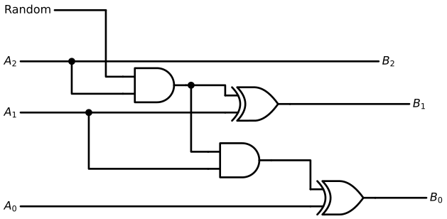
For the \(T\) gate, the operational principle is identical to that of the Hadamard gate, with an elegant asymmetry:
The \(|0\rangle\) manifold (\(A_2 = 0\)): Exactly half of the cube vertices map deterministically onto another vertex without any phase splitting.
The \(|1\rangle\) manifold (\(A_2 = 1\)): The remaining half of the vertices map into an equal superposition between real and imaginary phase axes (\(\frac{1}{\sqrt{2}} (1 + i)\)).
Just as we did for the Hadamard circuit, we can employ our balanced Random protobit source to govern the superposed states—except here, the stochastic splitting is applied conditionally.
# Initialize schematic drawing for the quantum T gatewith schemdraw.Drawing() as d: d.config(fontsize=12, unit=2.5)# Vertical coordinates for the input/output rails y_rand =5.0 y_a2 =3.5 y_a1 =2.0 y_a0 =0.5 x_in =0.0# ==========================================# 1. Place Logic Gates# ==========================================# First stage: AND gate for conditional imaginary phase toggle# Inputs: A2 and Random and_phase = d.add(logic.And().right().at((3.0, 2.8)))# XOR gate for B1 = A1 XOR (A2 AND Random) xor_b1 = d.add(logic.Xor().right().at((6.0, y_a1+0.25)))# Second stage: AND gate for sign flip when rotating from +i to -1# Inputs: (A2 AND Random) output and A1 and_sign = d.add(logic.And().right().at((5.5, 0.6)))# XOR gate for B0 = A0 XOR (Sign toggle) xor_b0 = d.add(logic.Xor().right().at((8.5, y_a0 -1)))# ==========================================# 2. Wire Random Input Line# ========================================== d.add( elm.Line() .right(1.5) .at((x_in +1, y_rand)) .label("Random", loc="left") )# Drop down into top input of and_phase d.add(elm.Wire("|-").to(and_phase.in1))# ==========================================# 3. Wire A2 Line (Presence / Control line)# ========================================== d.add( elm.Line() .right(10.5) .at((x_in, y_a2)) .label("$A_2$", loc="left") .label("$B_2$", loc="right") )# Tap A2 down into bottom input of and_phase d.add(elm.Dot().at((1.5, y_a2))) d.add(elm.Wire("|-").at((1.5, y_a2)).to(and_phase.in2))# ==========================================# 4. Wire A1 Line (Imaginary Phase bit)# ==========================================# From input to xor_b1 bottom input d.add( elm.Line() .right(2.0) .at((x_in, y_a1)) .label("$A_1$", loc="left") ) d.add(elm.Dot().at((2.0, y_a1)))# Tap A1 down into bottom input of and_sign d.add(elm.Wire("|-").at((2.0, y_a1)).to(and_sign.in2))# Main A1 path to xor_b1 d.add(elm.Wire("-|").at((2.0, y_a1)).to(xor_b1.in2))# Route and_phase output to xor_b1 top input and tap to and_sign top input d.add(elm.Wire("-|").at(and_phase.out).to(xor_b1.in1)) d.add(elm.Dot().at((5.0, and_phase.out[1]))) d.add(elm.Wire("|-").at((5.0, and_phase.out[1])).to(and_sign.in1))# Output line B1 d.add( elm.Line() .right(3.5) .at(xor_b1.out) .label("$B_1$", loc="right") )# ==========================================# 5. Wire A0 Line (Sign Phase bit)# ==========================================# Direct line from A0 input into bottom pin of xor_b0 d.add( elm.Line() .at((x_in, y_a0 -1.25)) .to(xor_b0.in2) .label("$A_0$", loc="left") )# Route and_sign output into top pin of xor_b0 d.add(elm.Wire("-|").at(and_sign.out).to(xor_b0.in1))# Output line B0 d.add( elm.Line() .right(1.5) .at(xor_b0.out) .label("$B_0$", loc="right") )
In conventional quantum hardware, multi-qubit entangling gates are notoriously difficult to implement—they suffer from high error rates, crosstalk, and delicate laser/microwave tuning.
In our molecular protobit architecture, the situation is completely reversed: multi-qubit gates (SWAP, CNOT, CZ, and Toffoli) are often structurally simpler to build than single-qubit rotation gates.
Because our channels are already organized into discrete protobit buses, multi-qubit control reduces fundamentally to boolean routing, multiplexing, and conditional masking.
The SWAP Gate
The SWAP gate exchanges the quantum states of two qubits. In our architecture, no active logic gates are required at all: we simply cross the physical protobit lines.
In standard Dirac notation: \[\text{SWAP} |a, b\rangle = |b, a\rangle\]
In our 3-protobit representation, swapping two qubits \((A_2 A_1 A_0)\) and \((B_2 B_1 B_0)\) is achieved by routing the two 3-line buses across each other: \(A_i \leftrightarrow B_i\). It is a zero-gate, purely geometric operation.
The CNOT Gate (Controlled-NOT / CX)
The Controlled-NOT gate flips the target qubit if and only if the control qubit is in state \(|1\rangle\).
\[\text{CNOT} |c, t\rangle = |c, c \oplus t\rangle\]
In hardware, conditioning an operation on a control qubit is achieved by multiplexing.
Because the target operation is a bit-flip (our single-qubit Pauli-\(X\) gate, which simply inverts the target’s presence bit \(T_2\)), the control condition simplifies directly:
* The control presence bit (\(C_2\)) and the target presence bit (\(T_2\)) are fed into a single XOR gate (\(T_2' = C_2 \oplus T_2\)).
* The phase lines pass through unaffected.
A single boolean XOR gate fully realizes quantum entanglement between two qubits!
The CZ Gate (Controlled-Z)
The Controlled-Z gate flips the sign phase of the state \(|11\rangle\) while leaving all other basis states untouched. Due to quantum symmetry, either qubit can act as the control or the target:
In our framework, the Pauli-\(Z\) gate is an inversion of the sign bit (\(A_0\)). Conditioning this phase-flip on the co-presence of both qubits being in state \(|1\rangle\) is remarkably simple:
1. An AND gate detects the joint condition: \(C_2 \land T_2 = 1\).
2. The output feeds into a XOR gate on the target’s sign bit: \(T_0' = T_0 \oplus (C_2 \land T_2)\).
The Toffoli Gate (CCNOT / Controlled-Controlled-NOT)
The Toffoli gate is the universal 3-qubit reversible gate: it flips the target qubit if and only if both control qubits are in state \(|1\rangle\).
In standard quantum computing, compiling a single Toffoli gate requires at least 6 CNOT gates and several \(T\) gates, creating a massive decoherence bottleneck.
In our protobit architecture, expanding the control condition requires no quantum compilation overhead whatsoever:
* We simply cascade an extra AND gate to verify the second control line (\(C_1 \land C_2\)), followed by our standard target XOR gate (\(T_2' = T_2 \oplus (C_1 \land C_2)\)).
Adding control lines scales linearly and cleanly, bypassing the compiler bottleneck that plagues current quantum computers.
Square-Root Logic Gates
Fractional quantum gates—operations that perform half of a classical rotation, such as the Square Root of SWAP (\(\sqrt{\text{SWAP}}\)) or Square Root of NOT (\(\sqrt{X}\))—might sound exotic.
Within our discrete geometric framework, however, the exact same design methodology applies systematically:
1. Map the 8-state cube vertices across the inputs.
2. For transitions that do not land squarely on a single basis vertex, decompose the fractional rotation into an equal superposition of adjacent cardinal vertices.
3. Construct the corresponding boolean multiplexing circuit, using the internal Random protobit signal to balance the superposed branches.
The Square Root of SWAP Gate (\(\sqrt{\text{SWAP}}\))
In quantum computing (particularly in quantum dot and spintronic architectures), the \(\sqrt{\text{SWAP}}\) gate is exceptionally important: applying it twice performs a full swap (\((\sqrt{\text{SWAP}})^2 = \text{SWAP}\)), but applying it once generates maximal quantum entanglement between two qubits.
In the standard computational basis \(\{|00\rangle, |01\rangle, |10\rangle, |11\rangle\}\), its unitary matrix is:
Notice its operational behavior:
* The identical states \(|00\rangle\) and \(|11\rangle\) remain completely unchanged (pure identity mapping).
* The anti-parallel states \(|01\rangle\) and \(|10\rangle\) are transformed into an equal, entangled superposition of each other with a relative \(90^\circ\) phase shift:
In our dual 3-protobit architecture (\(A_2 A_1 A_0\) and \(B_2 B_1 B_0\)):
Detection: An exclusive condition (\(A_2 \oplus B_2 = 1\)) identifies when the two qubits differ in presence (\(|01\rangle\) or \(|10\rangle\)).
Conditional Mixing: When this condition is met, our Random stochastic source triggers an equal superposition switch between crossing the lines (\(A \leftrightarrow B\)) and leaving them straight (\(A \rightarrow A, B \rightarrow B\)).
Phase Imprinting: The complex coefficients \(\frac{1 \pm i}{2}\) correspond directly to our \(T\)-gate phase logic, shifting the imaginary protobits (\(A_1, B_1\)) and sign protobits (\(A_0, B_0\)) into relative quadrature.
What is ordinarily treated as an elusive continuous quantum interaction is thus realized as a conditional, stochastic half-crossing circuit built from elementary boolean gates.
Reconstructing a Continuous Qubit from the 3-Protobit State Vector
Now, let us reverse the mapping: given a normalized \(1 \times 8\) protobit transition matrix \(\mathbf{P} = \begin{bmatrix} p_0 & p_1 & p_2 & p_3 & p_4 & p_5 & p_6 & p_7 \end{bmatrix}\), how do we algebraically reconstruct the continuous quantum qubit state?
In Dirac notation, a general single-qubit ket \(|\psi\rangle\) is expressed as a column vector in the computational basis \(\{|0\rangle, |1\rangle\}\):
The algebraic reconstruction operates across three direct steps:
Step 1: Recovering Signed Amplitudes by Difference
Recall that each real and imaginary axis was split across two mutually exclusive channels: one for the positive magnitude and one for the negative magnitude.
We recover the signed scalar components directly by taking the net difference between adjacent protobit channels:
For the \(|0\rangle\) Component (\(c_0\)):
Real part: \[d_0 = p_0 - p_1\]
Imaginary part: \[d_1 = p_2 - p_3\]
For the \(|1\rangle\) Component (\(c_1\)):
Real part: \[d_2 = p_4 - p_5\]
Imaginary part: \[d_3 = p_6 - p_7\]
Step 2: Quantum Normalization (\(\gamma\))
Because a physical quantum state must obey the unit norm constraint (\(\langle\psi|\psi\rangle = |c_0|^2 + |c_1|^2 = 1\)), we compute the Euclidean scaling factor \(\gamma\):
\[\gamma = \sqrt{d_0^2 + d_1^2 + d_2^2 + d_3^2}\]
Provided the state represents a valid, non-zero physical distribution (\(\gamma > 0\)), this scalar rescales the components back onto the surface of the Bloch sphere.
Step 3: The Recovered Dirac State Vector
Combining the signed components and applying the normalization factor \(\gamma\) yields the complete quantum state in canonical Dirac form:
\[|\psi\rangle = c_0 |0\rangle + c_1 |1\rangle\]
where:
\[c_0 = \frac{d_0 + i \, d_1}{\gamma} = \frac{(p_0 - p_1) + i \, (p_2 - p_3)}{\gamma}\]
\[c_1 = \frac{d_2 + i \, d_3}{\gamma} = \frac{(p_4 - p_5) + i \, (p_6 - p_7)}{\gamma}\]
This mapping provides an exact, lossless bridge: any 8-channel protobit state vector collapses seamlessly back into its continuous complex Dirac counterpart \(|\psi\rangle\).
Circuits de mesure
Échantillonage
Recuit Simulé
Exemples classiques
Retour de phase quantique.
Transformations de fourrier quantique.
Speculations & Wild Thoughts
Beyond Statistical Sampling: Can We Do Better?
Reconstructing continuous qubit amplitudes by statistically sampling over millions of discrete 3-protobit observations feels like an engineering concession. It mimics the clumsy “shots” measurement bottleneck of classical quantum simulators.
In a real, physical molecule, \(\pi\)-electrons do not roll dice to calculate their ground state—they settle via continuous, collective wave relaxation. There must be a more native, analog readout mechanism that bypasses statistical sampling altogether.
The 4-vertex tetrahedral POVM of QBism remains conceptually tantalizing:
* It requires only 2 protobits instead of 3.
* The probability conservation (\(\sum p_k = 1.0\)) emerges naturally and symmetrically from the geometry, without requiring separate longitudinal and transverse partitioning.
The catch? The operator matrices.
When you translate continuous quantum gates (like Hadamard or Phase rotations) into the tetrahedral basis, the resulting transition operators are not strictly stochastic: they become quasi-stochastic. To account for quantum interference, some transition elements dip below zero!
Because our molecular framework operates strictly on real, non-negative transition matrices (\(P \in [0, 1]\)), standard classical transition algebra cannot natively swallow quasi-stochastic operators without introducing complex canceling pathways.
We are standing at a theoretical crossroads:
* Do we embrace the 3-protobit Cube, which is 100% digital, non-negative, and easily wired with boolean gates at the cost of an extra spatial channel?
* Or is there an unmapped transformation that allows 2-protobit Tetrahedral manifolds to bypass quasi-stochastic negativity through topological resonance tricks?
The geometry of information is far richer than textbook quantum mechanics suggests. The quest continues!


 Speculations & Wild Thoughts